Introduction

Below is a log of my daily progress, including: 1.) What I worked on today 2.) What I learned 3.) Any road blocks or questions that I need to get answered 4.) What my goals are for tomorrow During the beak, January 7th 1.) I worked on researching relevant information about music generation through deep learning, in pariticular, the application of LSTM-RNN (Long-short-term memory recurrent-net-work) in this field. I also began to learn the basics of deep learning by watching all videos in Andrew Ng’s Sequential Model section of his deep learning coursera course. 2.) I learned the mechanisms of RNN: inputting the information yielded from previous timesteps through various different “states” (i.e. cell states) and hyperparameters to the next timestep so that temporal characteristics and relationship are preserved during the training/learning process. In the fundamental example of text generation (text-level or character-level), unique elements in the sequence form the “vocabulary” (it sounds more like a glossary to me) of the inputs, from which one can one-hot encode the sequences to proccessible matrices to feed into the model. There is also a loss function, which is a measure of error between the predicted and target outputs. Usually, the target outputs are the same as inputs except they are one step ahead. For instance, when one attempts to train the RNN to learn the word “hello” with a example sequence of length 4, he would input the one-hot encoded version of ‘h e l l’ and expect the model to successfully predict ‘e l l o’ at corresponding timesteps (‘successful’ means the probability of the target output is the highest within the probability distribution that the model actually spits out). The loss function is usually minimized by stochastic gradient descent or batch gradient descent, which is in between the regular gradient descent and stochastic gradient descent. In the calculation of gradient at each timestep, the expansion of chain rule will involve all the previous parameters, at a high level, propagating information back all the way to the very beginning. This is called “backpropagation”. However, backpropagation can generate issues such as the vanishing gradient since a long product derivatives whose absolute value is less than one will converge to 0. LSTM comes in handy here to mitigate the risk of vanishing gradient by its mechanisms of three different gates, which altogether operate to selectively forget and remember information from the past for a relatively long period of time. 3.) Terminologies such as “epoch”, “batch-size”, “activation”, “cross entropy” and “soft max”. 4,) Goals for tomorrow: learn more about LSTM and specific python libraries which can enforce it. Start to plan on the blue prints of the project (like a method section). January 9t 1.) I yielded primilimary results from the 2 layer text-based character-level LSTM model. The music data is in ABC (a notation in ASCII format). So basically, I was trying to generate music with the methods of generating texts. The training took too long (from last year to yesterday night) and the preliminary results did not generate very melodious music. I speculate the problems were due to the fact that I did not clean my dataset and my algorithm was too inefficient on my local CPU to obtain a high accuracy in a short time. 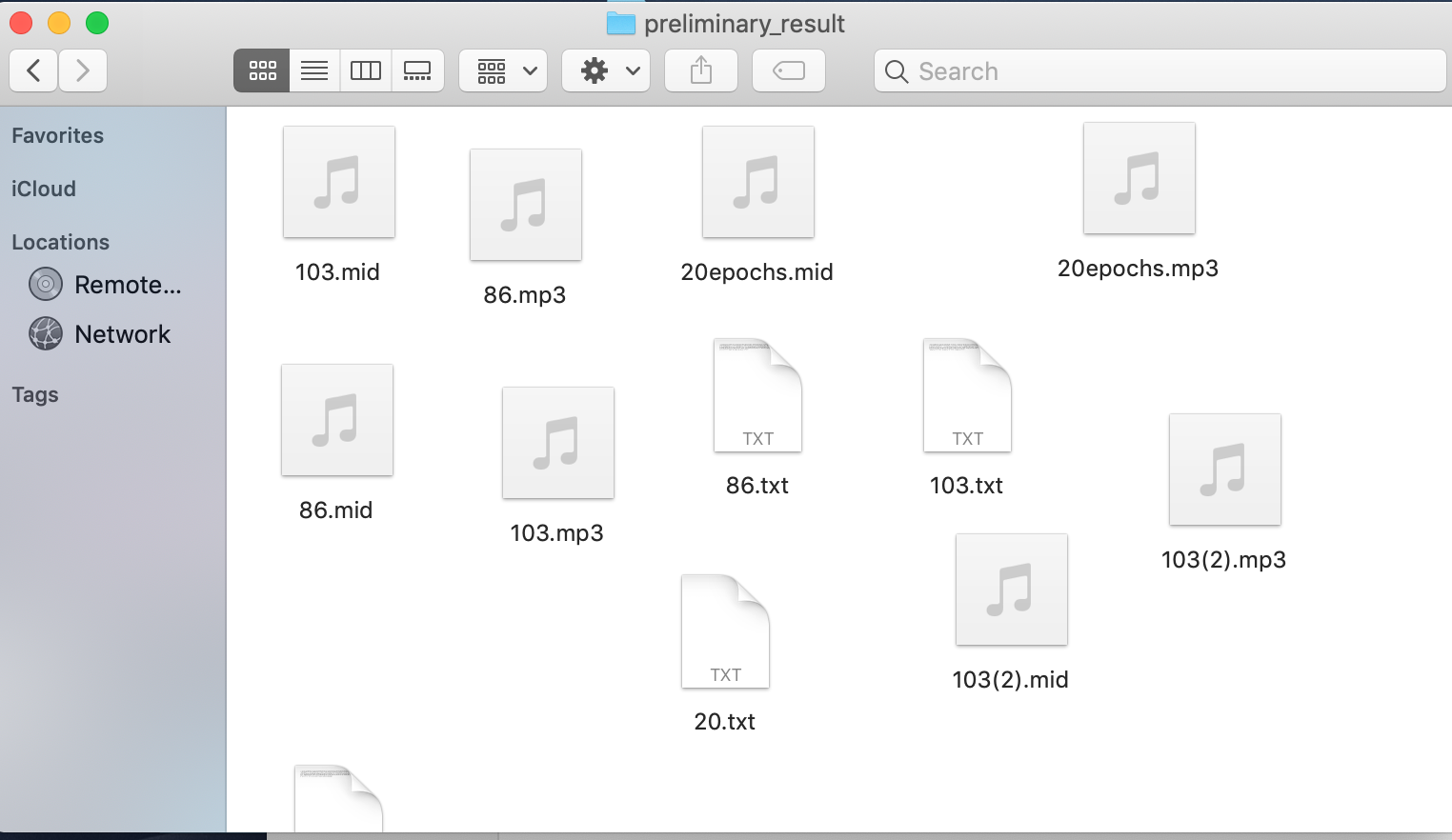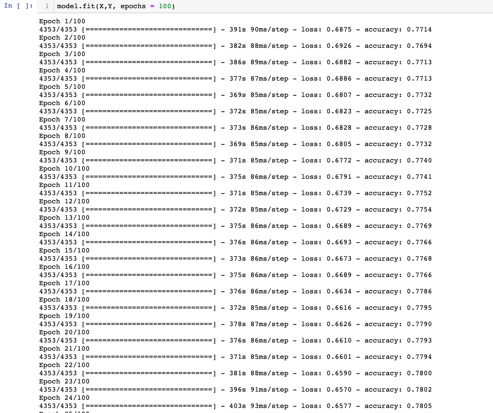Then I embarked on the Google Colab GPU to do a second version of this model. I also cleaned my data by deleting irrelevant lines such as titles and other descriptions, leaving only pure musical data. In Google cola, the model was trained super super fast. 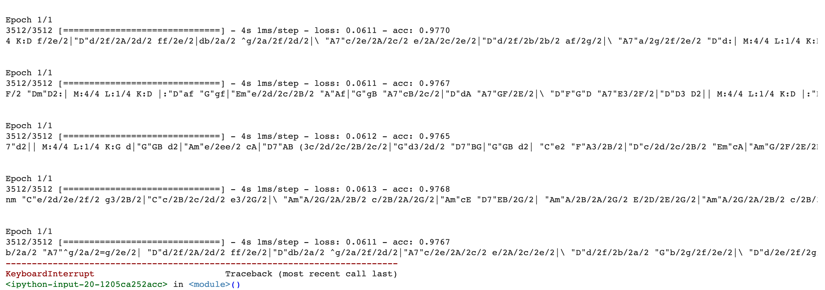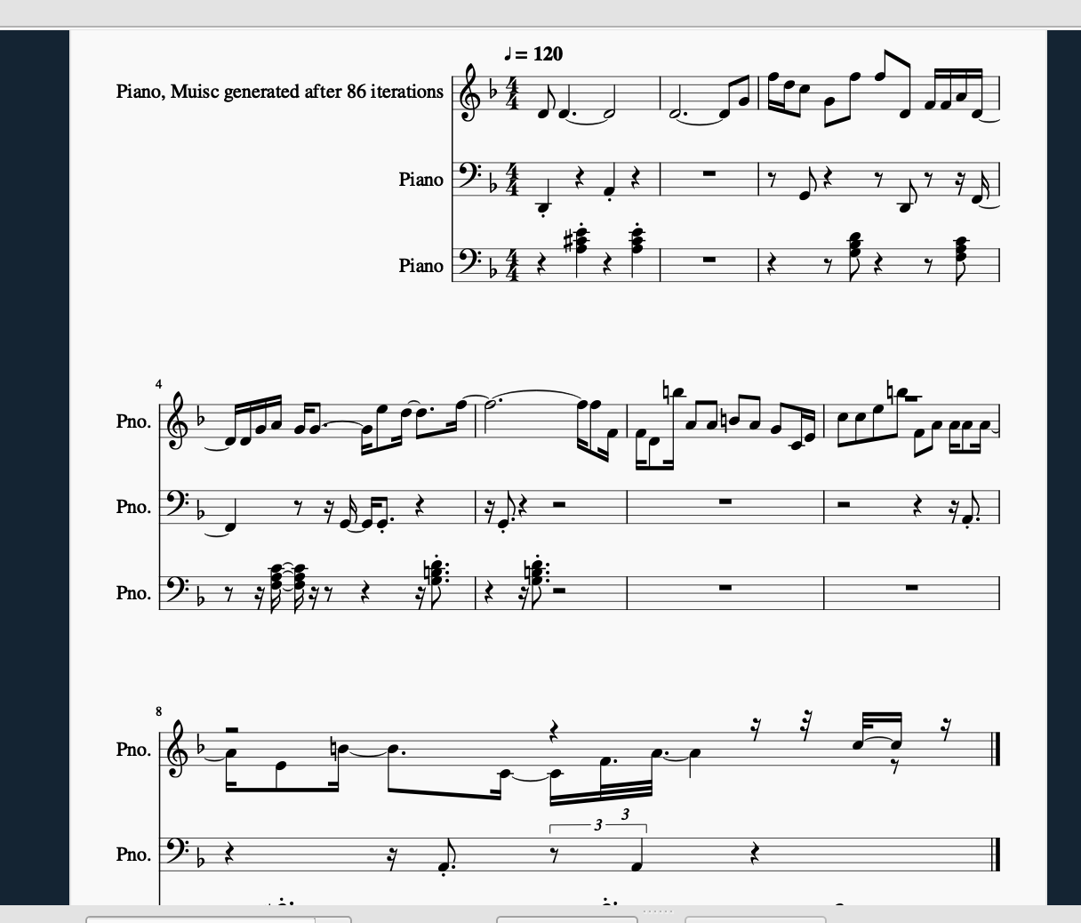Here are the training results: 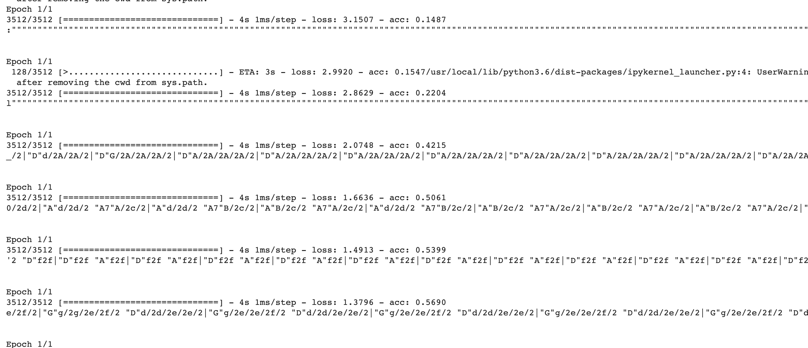Just by looking at it, you can see how the model starts from generating nonsense to well-structured ABC format notations. 2.) I learned how awesome these online GPU/TPU platforms like Google Colabs are! Also, I eliminate my confusions about the input/output shapes in the LSTM layers by reading from this source. In my particular many-to-many model, input and target sets should be in the exact same shape while the y_tn = x_tn+1. 3.) Everything went smoothly today and I did not encounter any road blocks 4.) Goals: start next part of my project. Generating music with other formats (like MIDI). January 10th 1.) I worked on preprocessing the midi data into matrix formats today. My codes were adapted from [here] (https://github.com/hedonistrh/bestekar/blob/master/LSTM_colab.ipynb). What this person does looks really interesting to me and his way of encoding a midi to matrix is analogous to how piano rolls and music box slits work. Following his methods, I successfully encoded Beethoven’s 32 sonatas into matrices. 2.) I learned what a RELU activation layer is and its advantage over sigmoid activation function in neural networks of many layers since it can avoid the vanishing gradient problem (the derivative of the linear and constant pieces will never change over long time steps). I also learned how to use the python library Music21 to process music information of a midi file, such as extracting note pitches, durations and offsets. 3.) I still need to understand attention layers which are shown in his code and other parts of that complicated architecture. I will probably use a self-coded simple one in my implementation. 4.) Goals: Start to train the model tomorrow on Google colab. 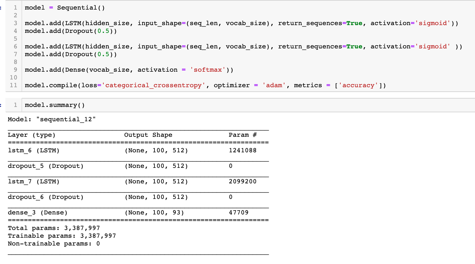January 13th 1.) I ran the piano-roll encoded midi model but unfortunately, the model performed nefariously terrible. The accuracy kept going down and the loss kept going up. I think that had a lot to do with the way I encoded the music data. There were too many 0s and since each music piece is in a different key, the matrix configurations were vastly different for the machine to learn. Thus, I gave up this method and decided to try another way of encoding only the information of pitches but not the durations and offsets, using a similar way of encoding language. I first extract all the notes and chords in the original Beethoven sonata midis, and I created a vocubulary consisting of unique notes and chords. The rest was just straightforward language last. Howevever, this time, instead of doing another many-to-many network architecture, I am doing a many-to-one model. Specifically, I use 100 notes to predict the next note. The input sequences were encoded into normalized vectors while the outputs were in one-hot forms. 2.) I learned how to create a many-to-one sequential model. 3.) I need to learn how different encoding methods of the same dataset can impact on the quality of model performance. 4.) Goals: get this part done during the weekend (training and generating music). January 15th 1.) I worked strenuously on finishing generating results using my MIDI LSTM. Although Google Colab runs so fast, it has many other aspects that drive me crazy. The notebook can only run for 8 hours and then it just automatically stops. All the memories and variables stored will get cleared up. For this reason, I retrained my models for a second time (wasting a solid 8 hour) and saved my model info to a h5 file. However, the load_file method for some reason is thrown away in the tensorflow 2.0 version, meaning that I can not open the model file I saved and downloaded either. Another full day of training became futile. Finally I found this super helpful online [article] (https://medium.com/@mukesh.kumar43585/model-checkpoint-google-colab-and-drive-as-persistent-storage-for-long-training-runs-e35ffa0c33d9), and deciding to add a checkpoint method in my training process and save modo info at each epoch along with the music generated every ten epochs in my google drive. But my google drive is too large to be mounted into a colab notebook (timeout errors). In the end, I literally created a new google account and had an empty drive just for this training. The training is still going and looks good so far. Hope this will work. And I tried the “load_weights” methods to test it out. Thank god tensorflow 2.0 did not abandon this method! I want to complain about 1 more thing, which is the OES WIFI. It shuts down at 11 pm every weekday and at 1 am on weekends! I can never train my models on google colab over night! 2.) I learned about the most CRUCIAL, PIVOTAL & QUINTESSENTIAL component of training a long neural network: callbacks! I have to save my model and model weights CONSTANTLY in order to be able to resume the training process without losing what is learned in case the run time stops or the kernel dies. 3.) I am kinda curious to learn why tensorflow disables so many fundamental methods like load_model in its new version. 4.) Goals: Really get the MIDI generation done and work with Daniel on the audio waveform generation part which is the hardest portion of this project. January 16th 1.) Daniel and I worked on the final part of the project: using audio waveforms to generate music. We worked on preprocessing music dataset by transforming each wav file to fft and we figured out how to write a new wav file using the inverse fft. 2.) We learned the usage of fast Fourier transform in audio engineering. 3.) Road blocks: we couldn’t find any fast ways to convert mp3 files to wav. So we needed to obtain a corpus of wav files somewhere. 4.) Goals: find the datasets of wav files! Start training as soon as we can! January 17th 1.) We extracted fft of 10 wav files, which are music composed by Saint-Saens. However, the files were too large to be processed on our local computers and even the 30GB memories of the Google colab. The system crashed for numerous time when we created the one-hot matrices of our y. Because there are too many unique values in our fft (over 68000000), the memories are so easy to run out. Then we decided to only use one song to train the model. But still, there is not enough memory. Finally we made a huge compromise, which is to feed the normalized fft vectors directly into the model without one-hot encoding the output. The model was literally a crap… We had a loss up to 350000… And the “music” generated was absolutely strident noise. So strictly speaking, we did not successfully complete this last part but at least at a conceptual level, we touched the ground of audio signal processing in python and learned the complexity and difficulty of deep learning tasks with waveforms as input materials. 2.) We learned to how to play around with the maximum memory of google colab and how to modify our model so that it could be compatible to pure vector forms of input and target. 3.) I want to know why there are so many unique values in terms of fft even if sometimes the same instrument was playing the same notes but at different time? 4.) Goals: write markdowns and explanations to our jupyter notebooks. Organize results. Make slides. Practice presentations.

This two-folded project uses various supervised binary classification algorithms to predict the for-profit or non-profit status of colleges as well as evaluates and digs into different factors relating to for-profit and predatory institutions in the higher education system. The data and explanatory variables were extracted and selected by Lauren from a governmental database.

This Regression Project did a series of analysis on the dataset of Happiness Scores of 157 different countries around the world in 2016. I picked the Happiness Scores as the response variable in my model. After seeing the bivariate associations between the response variable and all the other candidate explanatory variables, I decided to apply a multiple, RidgeCV linear regression model to my dataset. Before creating the model, I transformed one of the explanatory variables to its cube value to better achieve the assumption of linear correlation of multiple linear regression. Finally, I split the data into 70% : 30% and use the first 70% as my training/validation set and the rest as my test set. The outcomes appear to be pretty accurate and have good variability. You can find my code located here

The rollercoaster project extracted from HiMCM Contest 2018 the information of 300 rollercoasters around the world and did a series of analysis on various features as well as came up with our own ranking system. We examined the info of the whole dataframe and got rid of the columns with insufficient amount of data. Then, we filled in the few missing values in other columns with the mean of the rest of the data in the respective column so that we could do the further integrated analysis. We then asked several interesting questions regarding the age, geographical distribution and even the names of these rollercoasters. We plotted several graphs exploring the relationships among heights, lengths, and durations. Some interesting bivariate associations were discovered in this process. Then we tried to figure out the logics behind CoasterBuzz Rankings of the rollercoasters and did not find any reasonable explanations. Finally, we came up with our own equation of ranking based on our own preference.

Next you can update your site name, avatar and other options using the _config.yml file in the root of your repository (shown below).