Introduction

For our final project of this semester’s Machine Learning, we (Eric and Daniel) decided to generate music using LSTM neural networks. Deep Learning neural network was incredibly powerful in the domains of creating art. Famous works included generating Shakespeare-style sonnets and Harry Potter. In the music realm, AI compositions have also achieved great results such as Google doodle’s Bach’s chorales and the Magenta project. The year 2020 is the 250th anniversary of Beethoven’s birthday. A group of AI scientists started a project using deep learning to complete Beethoven’s unfinished Symphony No.10 in memory of this great composer and we are excited to hear the final outcome! So in the spirit of connecting science and art, which are the two immortal entities in this world, we start our journey to the area of music generation. And this blog post explains our first step to this journey.

LSTM

LSTM is a type of RNN (recurrent neural network) in sequence modeling which can keep learn-term dependency. Compared with the traditional neural network which an only process current information and input, RNN does a better job by remembering past information. This is necessary in generating texts and music since one needs to remember previous words in the sentence and previous notes in the music in order to generate a complete sentence or melody which makes sense. However, RNN has a problem called vanishing gradient that occurs when dealing with long sequences and using gradient-based method to calculate the loss. The internal mechanism of LSTM avoids this problem and can selectively remember and forget certain information from the past. Therefore, we chose LSTM as our general framework to generate music. If you want to really understand the details of LSTM, you can go to this post or this post.

Part 1: Text-based music generation

The first part of our project is music generation using music data documented in abc format. For non-musicians to understand this, it’s basically a text-encoded type of sheet music, which means that we can process music scores of abc format in the same manner we process strings and texts. And what we are doing here is essentially generating “texts” using a character-level LSTM and some/most of our generated texts are able to be further converted to standard music notation, MIDI or mp3 without any artificial edits. We acquired our datasets from the online Nottingham abc database. We collected over 1000 simple folk tones in a single txt file.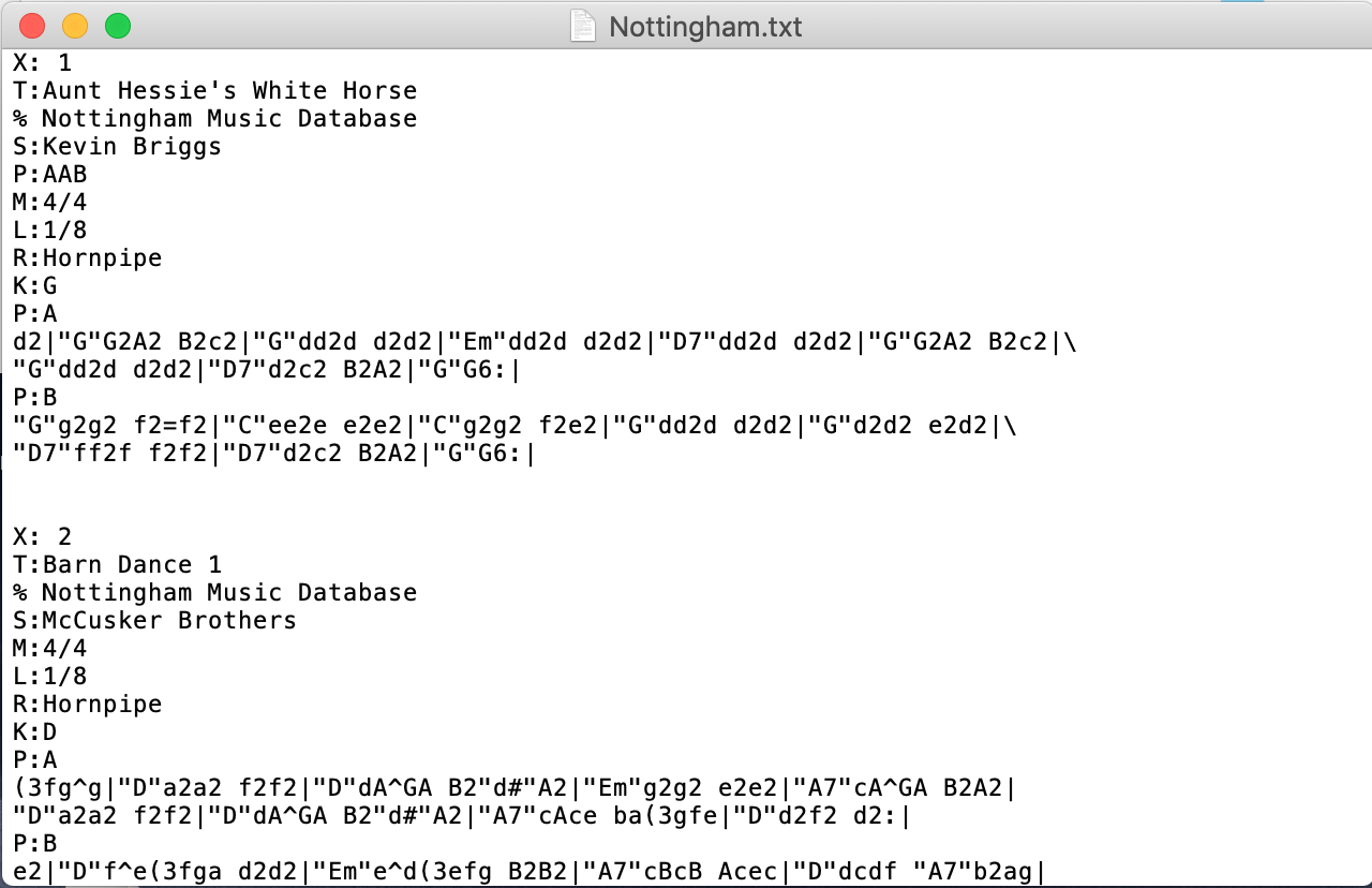

Preprocess

After we cleaned the dataset, we started to encode the data into processable formats. We decided to do a character-level LSTM. So we first created mappings that matched each unique character in our dataset to an integer. Then, we created our one-hot input and target sets. Since the model is many-to-many, the input and target sets have the same shape. In fact, target set is just one character ahead so that the model is always trying to predict the next character. The sets contained sequences of length 100.

Model

After several trials, we used the architecture below for our formal text-based generation task: 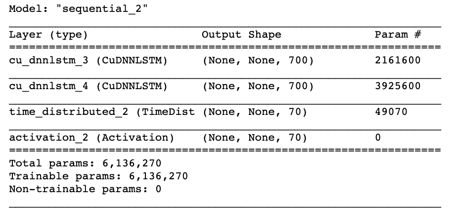The CuDNNLSTM is a much faster LSTM that can be run on a GPU environment (for this project, we used Google Colab’s GPU). There are two layers of LSTM. We use return_sequences=True for stacked LSTM. And we finally dense the output to the shape we want.

Training and generating text

This is the most wonderful part! I wrote a function to generate text of any length you want, and this function is called after each epoch of the training to see if our model is getting better and better at generating abc format music.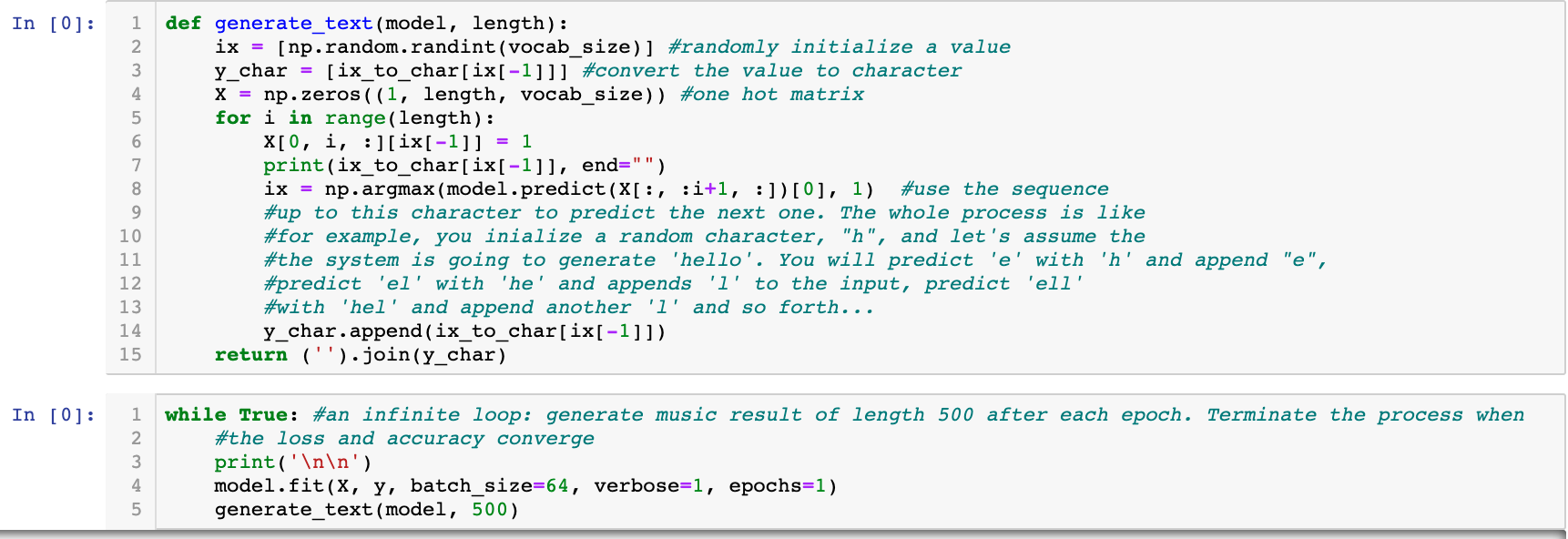

I was very much amazed by how fast this could run! (4s/epoch)

As you can see, the model seemed to learn the format of abc notation (such as time signature, key, and measure lines) by itself pretty amazingly. . Here is one example of generated txt: 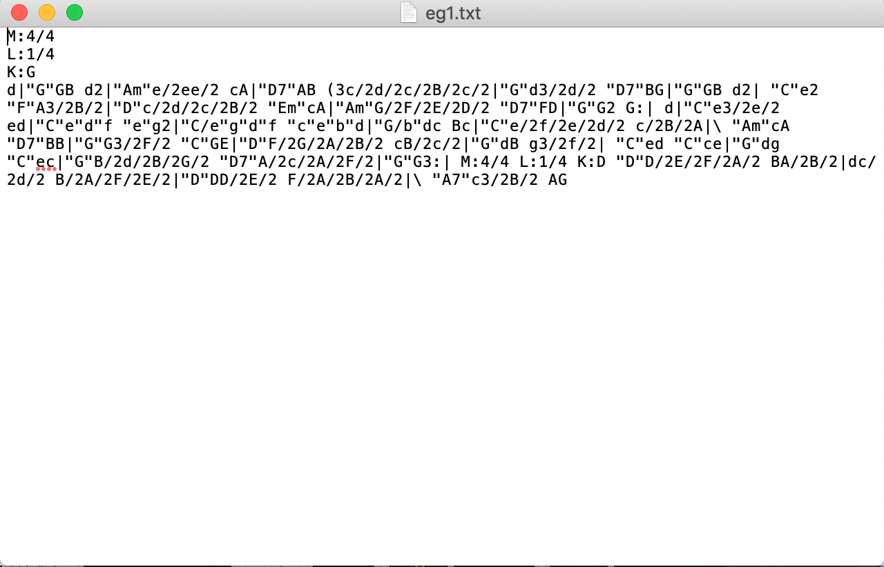We could convert this txt to midi just by copying and pasting it to this website. And it looks like this in standard music notation: 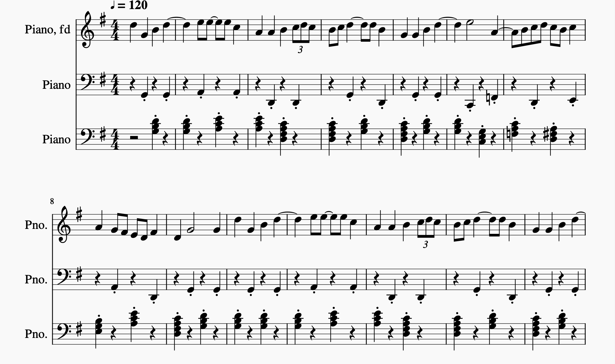. You can also listen to it! Harmonically, it follows the tonal structures very well. There were even very few wrong chords. The melody sounds pleasantly simple. And I believe it’s very hard for non-musicians to differentiate it from human-composed music since it has a melodic theme that is recurrent! One picky comment I would make is that the measure line seems to be placed one beat off. But who cares? However, I am a little worried that it might be too good that it was overfitted. I hope in the future when doing similar tasks, I can find a way to evaluate the similarity level between the result and the original dataset. It’s still very cool even if it just reproduces a song or several segments of different songs in the original dataset. This potential problem of overfitting made me decide to use dropout layers in the next part to automatically turn off some cells so that not everything would be learned.

You can find our code for part 1 here

Part 2: MIDI-based music generation

In this part, we directly used MIDI format data to generate music! We acquired our dataset from the kunstderfuge MIDI database and downloaded the midi files of the 32 piano sonatas of the greatest Ludwig van Beethoven. They are the New Testament for pianists!

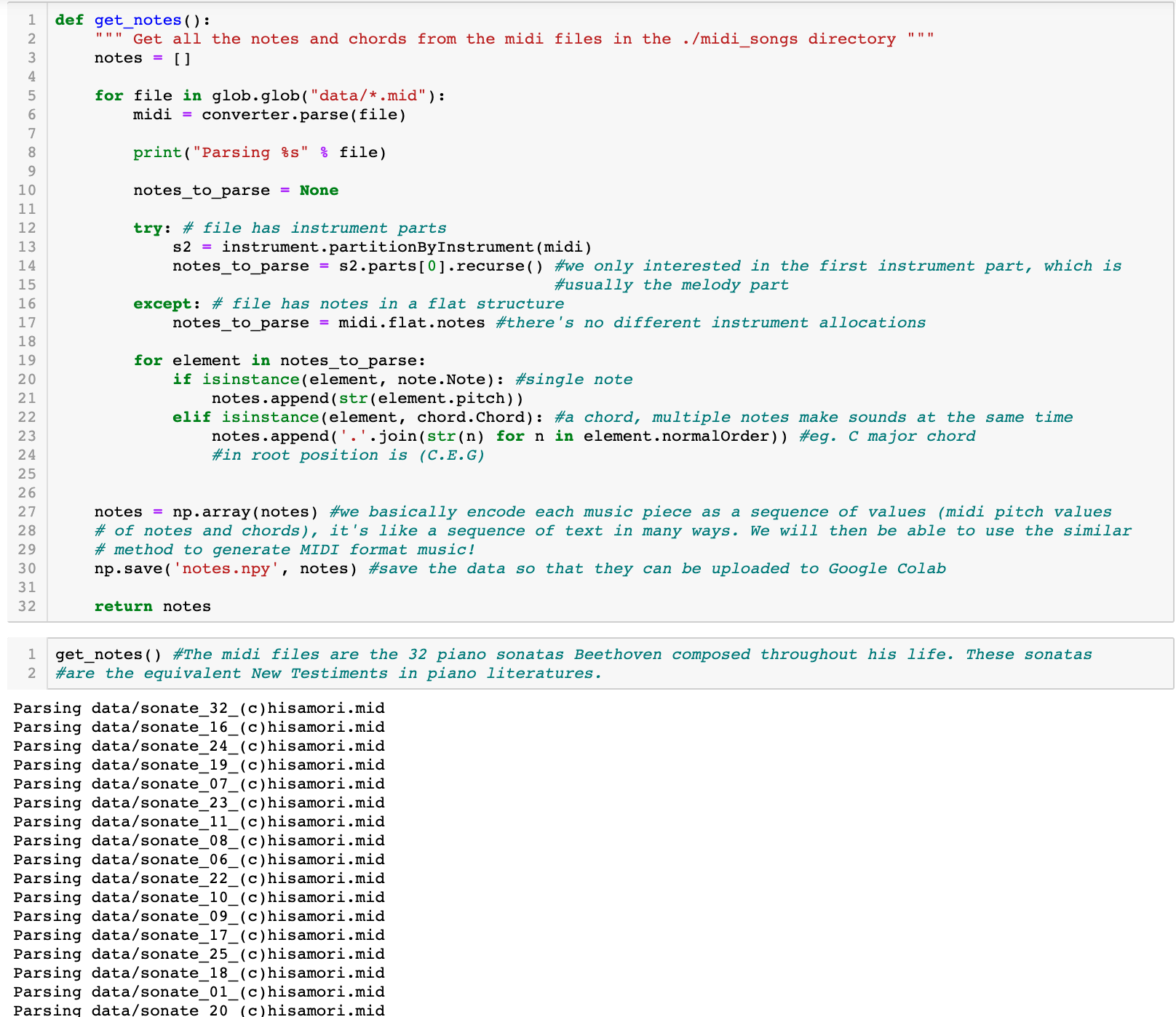
Preprocess

We extracted only the pitch information (not durations or offsets) of the music and we represented all data in an array of midi pitch values. For chords, we just bundled all the different pitches together joined by a period. The rest was all same as what we did in Part 1 such as creating mappings with integers. But what’s different this time was that we used a many-to-one instead of a many-to-many model. We were only predicting the 101th note given the first 100 notes of a melody. So we only one-hot encoded the target set and directly fed the normalized input set to training.

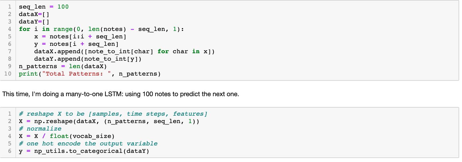
Training and generating midi

The training process this time was much more painstaking since there was much more computational load and the runtime in Google colab shut down for different reasons. I learned that it’s always important to create a callbacks calling in the model.fit part since it allows you to save the weights of the current model as you train it. We can always resume the training process instead of starting over when we have this. So once again, very important: Callbacks, callbacks, callbacks!!!

The architecture is as follows:

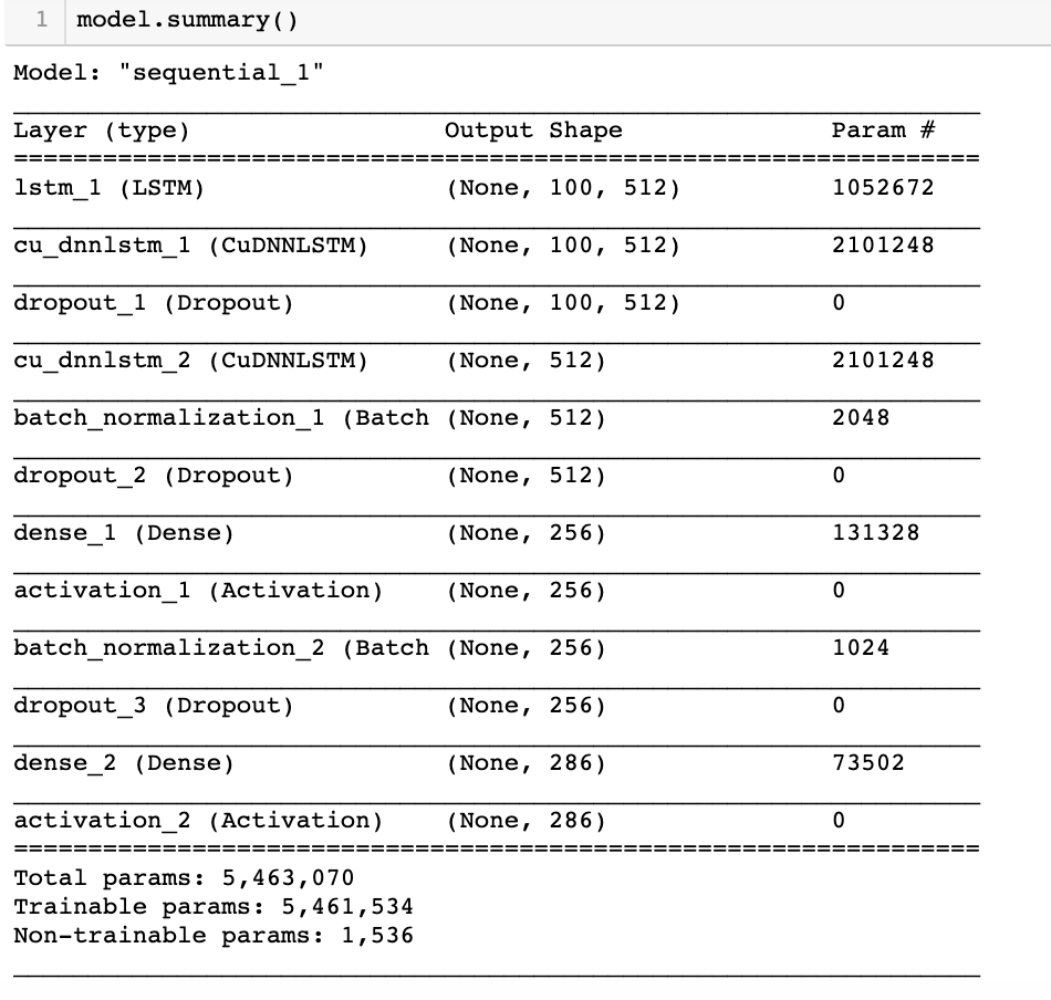
There are three LSTM layers, and in between are drop out layers which randomly turned off 30% of cells to avoid overfitting. The sequence was not specified in the model this time cause we wanted to generate a melody note by note using all the notes already generated. A new piece of music was generated every 10 epochs.

Here is an example we generated after 110 epochs.

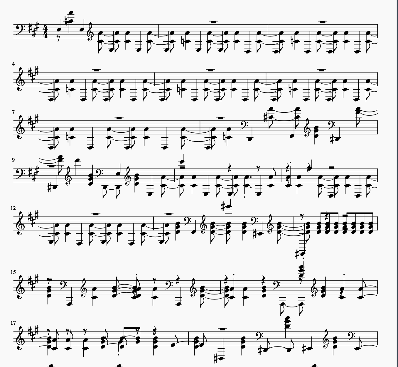
You can listen to it here

Well it looks much less neat and crams all the parts (accompaniment, melody) all together. This makes sense because that’s how we extracted notes and chords in the first place. And since we did not keep any information regarding the durations and offsets in our preprocessing, all notes were set to eighth notes. Frankly speaking, it sounds not bad and much more “original” though mechanical and metronomical. You can hardly trace any Beethoven’s phrases here. Although, musicologically, there were many counterpoint errors and wrong chords. I was fascinated by many repeated spots in the music. It almost sounded like our model went to an infinite loop but magically it could find its way out. For me, the style of this piece is more akin to the contemporary minimalism music than Beethoven’s sonata. Perhaps the underlying nature of Beethoven is actually Philip Glass? (It’s kinda sacrilegious to say that as a classical pianist).

You can find our code for part 2 here

Part 3 : WAV-based music generations

The last part is our most challenging and least successful attempt to generate music from audio wav files. This method is completely musicological illiterate compared with the previous two, which to some degrees, both contain musical knowledges such as chord and pitch names. Wav files are waveform representations of sounds, which are the most fundamental and natural type of representation. In theory, under the most idealistic condition, if a neural network is able to fully “learn” the waveforms and produce a new wav file containing features of the trained wave forms, a new piece of “music” can be created. Different from the previous two methods which can only learn information about pitches, durations and offsets, the waveform-based music generation method is possible to also learn the timbre and loudness of sounds, the so-called “expressive” elements in music. But the actual implementation is far more intricate than the rationale. It is actually “devilishly hard”.

Preprocess

Before we got our hands on actual music wav files, we first learnt about the application of wav signal processing in languages. Instead of directly tracing the patterns in the time domain waveforms (a sound wave graphed in intensity/loudness v.s. time coordinates), most research utilized Fast Fourier Transform (FFT) to preprocess the signal to extract major frequencies in the beginning. The greatest usefulness of FFT is its ability to extract major frequencies out of a complex waveforms. It is kind of analogous to the ability of separating different colors from a muddy pond of miscellaneous pigments. It considerably reduces the variability in the wav files and retains the most important information in the signals. And the FFT in python is actually coded using the formula of discrete Fourier transform (the equation of the wave are too complex or unknown, it is very hard to compute a complex integral from negative to positive infinity using the wave equation), meaning that we approximate the Fourier transform of the original wave using a finite number of points on the wave sampled. FFT signals (magnitude vs frequency) can be turned back to waves in time domain using inverse FFT (IFFT). The equations of discrete FFT and IFFT are below:

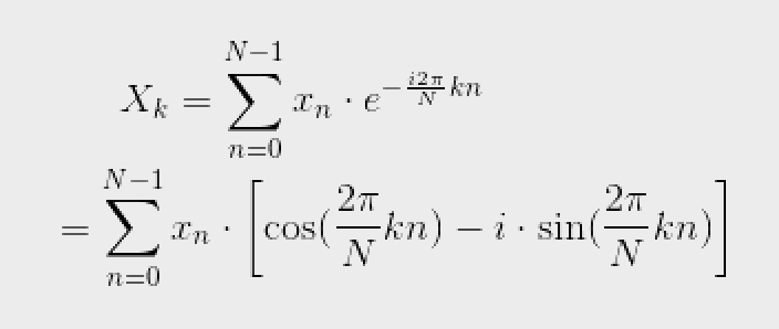
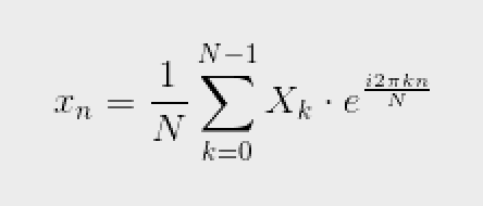
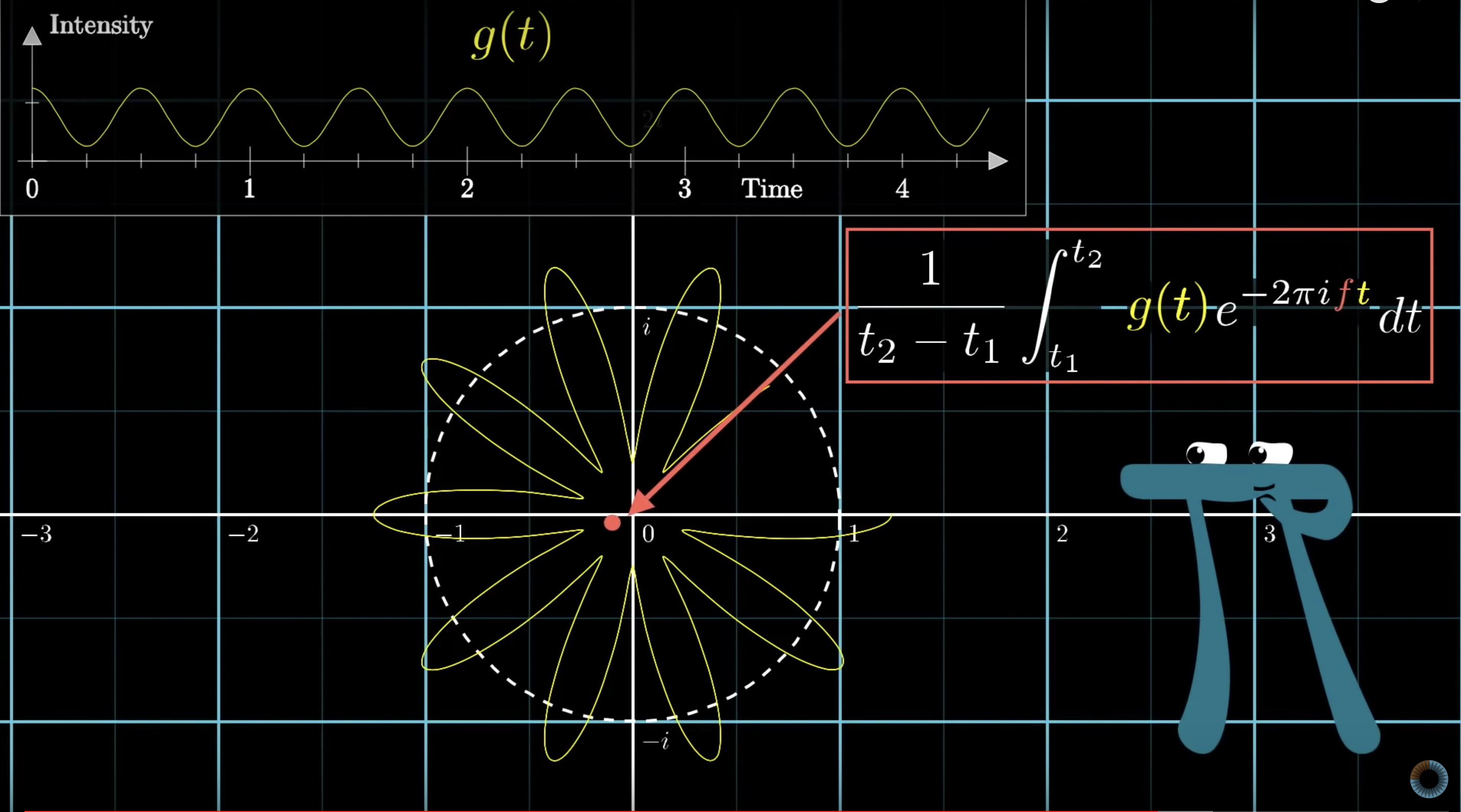
Note the Euler’s formula part in the FFT equation, which hinted at the concept of rotation in a complex plane. In fact, 3blue1brown has a video demonstrating a visualization of FFT as waves “winding up” at a particular rate around the circle and the center of mass of the graph traces a factored form of FFT graph. It is really fascinating! However, this is not a calculus blog post and our understandings haven’t reached the depth to explain the mathematical nature of FFT yet, we are just going to use it anyway.

We tried a speech wav file of a 5s English phrase to on the FFT and IFFT methods in python, and were successfully reproducing a new wav file sounding very close to the original one (though a little bit distorted) with recognizable speech content. So we “FFTed” the wav files of 10 different music of Saint-Saens in similar manners. `

But this is where we messed up:

The fft vectors were so absurdly large that when we tried to create a vocab list of unique frequency values among the 10 different songs the nearly 30GB RAM of google Colab always crushed, for over 10 times. Then we alleviated the burden by using a single song only. But still the RAM crushed. The data size and the vocal size were nearly identical, meaning that almost all frequencies are themselves unique. It is like writing a long essay but each character in it is a different one. So it’s enormously diverse and wild for a neural network to learn. The only way to keep it alive was to NOT one-hot encode the targets (which is technically not okay since the correspondence between encoded value and index in the matrix is lost). So the whole started to make no sense from here…

Training (messing around) and reflection

Anyway we still wanted to make something audible from here!! We basically just made some adjustments in the dimensions and applied the MIDI LSTM model to the data. The loss skyrocketed to over 30 million and there was literally no accuracy (in the order of magnitude of 10^(-19)). And yes, we did write an audio file from the output after just 1 epoch. It is absolute noise and we feel deeply sorry for Camille Saint-Saëns…

But it’s really worth thinking that there is so much frequency complexity just within a single short piece of music that it is too large to be processed in the same manner as we process the whole volumes of Shakespeare’s texts and even the whole set of Beethoven’s 32 sonatas (24h full length if you were to play the whole set on the piano). The extra, nuanced details wave files captured are obtained at the expense of exponentially increasing the internal entropies of the inner contents. And that’s probably why existing studies mostly used wav files to generate sounds of new timbres but seldom attempted to generate music with raw wav files.

This last part was definitely beyond our capabilities. We were overconfident and too idealistic and our final outcome was a joke… (WARNING: don’t listen to the noise file, it can be detrimental to your hearing and the acoustics of the computer’s amp) But we were satisfied to have learned a little bit about signal processing and its application with python packages in a short period of time.

You can find our code for part 3 here

A few words to say in the end (Eric)

This is totally non-technical.

Growing up as a musician, I never seriously pondered over the nature of music. As this project has demonstrated, music is simply a sequence of discrete events occurring in time. But can we REALLY understand music by finding the curves of best-fit of high dimensional distributions? What’s the “hidden state” behind Beethoven’s genius? Are AI-composed musical pieces the miraculous creations of technology or ridiculous imitations of human works? How does the machine know what note is the right one to play? How do we know what note is the right one to play?

I feel very fortunate to be a musician and be able to detect and identify different pitches coming from different instruments when listening to a symphony. Just think about it, every second, my brain is doing Fast Fourier Transforms over these complex signals by itself!